-
Property & Casualty
Property & Casualty Overview

Property & Casualty
We offer a full range of reinsurance products and the expertise of our talented reinsurance team.
Expertise
Publication
Biometric Information Privacy – Statutes, Claims and Litigation [Update]
Publication
Inflation – What’s Next for the Insurance Industry and the Policyholders it Serves?
Publication
Human Activity Generates Carbon and Warms the Atmosphere. Is Human Ingenuity Part of the Solution?
Publication
Illinois Changes Stance on Construction Defect Claims – The Trend Continues
Publication
Generative Artificial Intelligence in Insurance – Four Aspects of the Current Debate
Publication
Battered Umbrella – A Market in Urgent Need of Fixing -
Life & Health
Life & Health Overview

Life & Health
We offer a full range of reinsurance products and the expertise of our talented reinsurance team.

Publication
Underwriting High Net Worth Foreign Nationals – Considerations for U.S. Life Insurance Companies
Publication
Group Term Life Rate & Risk Management – Results of 2023 U.S. Survey
Publication
Trend Spotting on the Accelerated Underwriting Journey
Publication
All in a Day’s Work – The Impact of Non-Medical Factors in Disability Claims U.S. Industry Events
Publication
Marginal Gains in the Medicare Supplement Market -
Knowledge Center
Knowledge Center Overview

Knowledge Center
Our global experts share their insights on insurance industry topics.
Trending Topics -
About Us
About Us OverviewCorporate Information

Meet Gen Re
Gen Re delivers reinsurance solutions to the Life & Health and Property & Casualty insurance industries.
- Careers Careers
AI-Based Pricing of a Disability Income Product

May 07, 2020
Dr. Behrang Jalali, Karin Brendel
English
In today’s framework of digitalization and technological disruption, capturing most relevant and high-quality data, while complying with customers’ data privacy as well as ethical and legal aspects, and employing advanced analytics techniques – implemented with the right infrastructure – are key in ensuring best customer service and moving forward in line with the current AI developments.
To follow through with this goal, and to differentiate hype from real business-applicable solutions, it is fundamentally important to design analytics projects from the beginning in a comprehensive manner.
In short that means starting with a broad data collection and revisiting data processing through constructing models, taking into account various performance evaluation measures, and continuing all the way through to consistency checks of the model predictions, as well as frequently aligning with insurance expertise from various areas.
In this article, we describe the implementation of one specific project, focusing on a narrow AI application, that uses machine learning in a supervised learning approach. Our application showcases pricing of Disability Income business. We present an end-to-end journey of how such a set up works, taking you through all the steps required and highlighting where business experience and expectation can influence and co-evolve with the AI-based pricing outcome.
As Andrew Ng, the co-founder of Google Brain and the former chief scientist at Baidu, highlighted in a 2019 Harvard Business Review article, AI projects can add value in three ways: 1) reducing costs by automating tasks, 2) increasing revenue by prediction systems, and 3) launching new lines of business or products that were not possible before.
The approach we show here contributes value in all of three aspects Ng identified: the pricing approach outlined shows a way to build the foundation of more automated tasks with fewer manual adjustments. Also, it highlights possibilities for more personalised offers with premiums that are commensurate with the individuals’ risks. Lastly, it shows ways to further explore areas for premium differentiation or unification – by defining segments of customers with similar risks in new ways – based on the data that has been collected.
Traditional pricing approaches
Life actuaries have been analysing portfolio or population data for decades and derived probabilities for mortality or morbidity. As long as these rates were differentiated by “Age” and “Gender” only, actuaries could endeavour to build up the sufficient data volume to estimate these probabilities from the raw data, splitting the data for calculation of rates for males and females and smoothing the raw values.
However, mortality and morbidity rates are a function of a vast number of lifestyle and genetic factors. In the insurance context, some of these have been measured, recorded and increasingly used in pricing – first based on expert opinion but increasingly based on emerging data related to these variables. Examples include variables related to occupational risks, wealth and the health status at policy inception or the time elapsed since then.
Thus, actuaries create high-dimensional datasets with substantial correlations between the variables of interest and a varying volume of observations for all possible combinations of these variables.
Due to the correlations, unknown in extent if not in nature, deriving insight from the raw data, filtered by the variables of interest is not sufficient anymore. While this step is definitely part of any analysis, it is considered as only the first step in exploring the data.
Hence, constructing multidimensional models to describe the data is necessary. Nevertheless, it comes with some challenges:
First, observational data is determined by the insureds under risk in a given period of time (i.e. exposure) and the respective events of interest for Protection business, i.e. the death or disability claims, which are very rare.
The variables selected and their sublevels (possible values of a categorical variable) determine the number of combinations for which the mortality or morbidity rate needs to be determined. But those combinations can easily reach millions or billions, which makes credible predictions for rare observations impossible.
Secondly, GLMs (Generalised Linear Models) have been used for modelling mortality or morbidity rates, but their usage comes with some drawbacks: While an assumption of Poisson-distributed events might theoretically be applicable, actual datasets can be found to violate that assumption. Using discrete variables as numerical will only follow exponential patterns, which is too simplistic for a variable like “Age”. Transforming discrete variables to categorical ones is a far from an ideal solution to this, which goes along with ignoring important information, drastically increasing the dimensional space of the modelling exercise and losing interpretability options. Also, GLMs can reflect interactions but only if known and explicitly determined beforehand.
Given the complex high-dimensional datasets that actuaries usually encounter, using complex multidimensional models – in our case, Gradient Boosting Machines (GBMs, an ensemble of decision trees) – seems the natural solution. This has become possible thanks to increasing computational performance and available software.
Yet introducing AI to pricing is not only replacing simpler algorithms with more sophisticated ones, but also designing a whole new approach that aims to build a data-driven process, as in this application for the pricing of a Disability Income product. There is a fundamentally important difference in an open-ended approach, experimenting with a multitude of models and selection of variables as broad as possible. Narrower approaches, if only limited by past computational performance issues, are prone to strong confirmation bias. In other words, by shaping and preparing the data and their correlations mainly based on actuarial expectations, we lose the chance to detect unknown patterns or explore new relationships – which advanced models can detect or highlight for further exploration.
The data and the business objectives
In the use case at hand, we focus on modelling incidence rates of Disability Income Protection business. The experience data we used covers nine calendar years; with sufficient exposure years and claims (including incurred but not reported) to perform thorough modelling. We defined incidence rates as number of claims (counts) divided by exposure, to be the response that we aim to model. Among the common pricing variables are:
- Age (from 20 to 60 years)
- Gender (Male and Female)
- Occupation class (from 1 to represent least risk to 10 as highest risk)
- Calendar year (2008–2016)
- Selection year (split into the first nine years separately and ultimate beyond)
- Benefit or sum insured (very small, small, average, high, very high)
Please note that the patterns shown here are of illustrative nature, we do not disclose the exact results of our experience analysis or all data specifications, but the data is typical of a long-term Protection business portfolio. Another example of such experience analysis can be found in Gen Re’s Dread Disease Survey.
The result of this modelling exercise is two-fold: By constructing and selecting the best multidimensional models to describe the data, we first generate insights that – in contrast to just looking at the data – take into account detailed relations among the variables. For instance, we can explore and truly investigate the following business questions with the confounding factors being considered appropriately:
- Is there a “Calendar year” trend?
- What is the extent of “Selection year” effect?
Second, we develop a model that calculates our best prediction of the incidence rates for any given combination of the variables. That means we can generate incidence rates for specific so-called model points – potential insurance applicants for the course of their policy, taking into account the selection effects in the upcoming years – and use these in our normal actuarial premium calculation tools. Thereby, we open up further possibilities for pricing Protection business with adequate premiums that are commensurate with the risk of the individual.
Analytics set up
In any modelling approach, a priori we cannot know which type of model will be most appropriate to describe the data and return a reliable outcome and with satisfactory performance. In this project, we have applied GLM and GBM algorithms. The basic GLM without regularisation served as the benchmark model. We compared it with GLMs with varying regularisation parameters and grids of GBMs to explore a wide range of values for its key parameters (as can be seen in the section with technical details).
Before we arrived at the preferred data structure as presented in the previous section, given the motivations described earlier, we experimented with several versions of aggregation levels. Too granular data led to unsatisfactory modelling results as the models picked up too much noise in the data. On the other hand, data with a too high-level of aggregation could not be used in differentiated pricing and would not generate valuable additional insights. The data selection and preliminary modelling process were carried out iteratively to strike the right balance of a stable model with sufficient performance on granular data that provides compelling insights and an interesting basis for refined pricing.
The final, selected data set was used with the resulting exposures, for all combinations of variables and sublevels, as weights in GLM and GBM modelling. To evaluate models, we measured their performance by metrics, by inspecting validation plots, which compare predicted versus observed incidence rates and by applying interpretability methods such as partial dependence plots. Thereby, we selected the top performing models based on their performance on the test, i.e., unseen data.
Modelling approach – technical details
With sophisticated algorithms – such as a highly performing GBM – and an open source, in-memory and distributed machine learning platforms – such as H2O – there is no need to manipulate data in an ad-hoc fashion or to assume specific interaction terms up-front. One can build numerous models of this algorithm, identifying a family of best models that can best describe prominent and detailed patterns in the data.
In a first step, we refined the benchmark GLM by introducing regularisation to GLMs, which (in short) is a penalty for additional variables if their influence on the response variable is of lesser degree. We used elastic net as regularisation approach, which blends two different types of such a penalty term, lasso and ridge regression. We varied both relevant parameters to improve the benchmark GLM and to systematically determine the right level of regularisation that achieves the best model performance on the test data.
Similarly, advanced algorithms such as GBMs, with flexible complexity, are sophisticated at learning detailed patterns in complex and high-dimensional data, but this comes at the price of adjusting many so-called tuning parameters to obtain the best results. One cannot know in advance the optimum values of a model’s parameters that lead to satisfactory performance for a given data.
Thus, it is necessary to construct grids of models, which basically means looping over a range of different values of each of the tuning parameters. In a simple approach, by choosing a metric such as the weighted MSE (Mean Squared Error, a metric that essentially measures the distance of predicted and observed points), we optimize models along the grid to identify top performing models.
Among the key tuning parameters of GBMs are: the depths of each decision tree, the learning rate (i.e. how fast each model approximates the improvement over previous trees), sampling fraction of data rows and sampling number of variables at each splitting node of a tree. In our project, small experiments with two additional parameters, namely sampling number of variables per tree as well as minimum number of rows at leaf, were essential in constructing stable models. Stable here means that the results did not vary substantially when the modelling was based on different seeds or different splits of the data.
Another fundamentally important criterion in machine learning is to monitor and correct for possible over-fitting; i.e. when a model learns the data in training steps very well but fails to perform similarly well on a test data. Using H2O, we have applied “early stopping” (simply speaking, adding conditions to stop a model improving too much in training steps) to control this effect. We monitored the resulting performance on train and test data to identify optimum areas of the parameter space, which led to best and sufficiently general solutions.
Model evaluation and selection
Constructing a variety of GLMs with different regularisation parameters and the grid of GBMs, we used statistical metrics as a first step to identify top performing models. For those, we have evaluated the so-called validation plots to compare predicted and observed values in a second step.
As the “Age” variable is the most relevant predictor in Protection products, we highlight it in an example of one of the best models for the variables “Age” and “Gender” in Figure 1. Bear in mind that we have modelled all variables at the same time in this model, but here we depict the predicted shape of incidence rates in terms of these two variables.
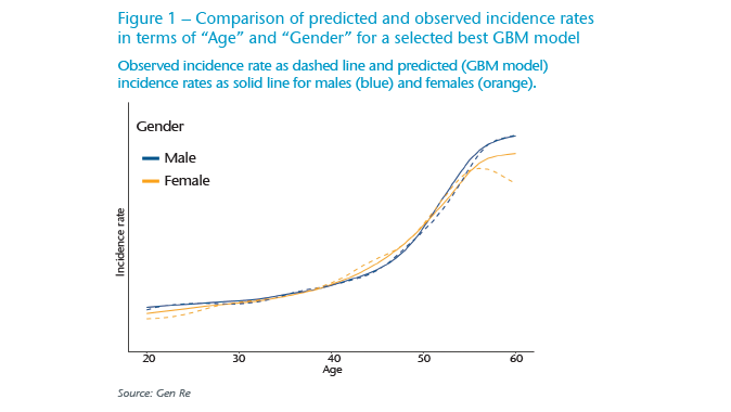
The comparison shows that this selected GBM is closely describing the observed data. The drop in the observed values for females beyond the “Age” of 55 as shown by the yellow dashed line, is a common observation but is rather an effect of skewed or scarce data in that range – it is not considered a real pattern. Considering this, a rise in the modelled female group, shown in the yellow solid line and similar to the pattern in the male group (blue solid line) is a more realistic prediction.
For the top performing models identified by a statistical metric, we inspected the validation plots for all variables. Thereby, we convinced ourselves that a top range of models looked consistently satisfactory for all variables and performed similarly well.
It is noteworthy to mention that it is not possible to achieve a similarly good performance in such a validation plot for “Age” and “Gender” with GLM models without converting “Age” to a categorical variable; however, this has other disadvantages as mentioned earlier.
Overall, we noticed that compared with GBM models, various GLM models with different regularisation parameters did not improve much over the benchmark GLM and could not achieve the same performance as the selected best GBMs. Therefore, in the following sections we focus on the results of the GBMs.
Interpretability methods – verifying trust and transparency
Beyond optimising grids of models based on typical statistical metrics and inspecting top performing models in validation plots, such as the one shown in Figure 1, it is necessary to evaluate the outcome of machine learning models a bit further – especially before deployment.
Applying interpretability methods is another angle for assessing the performance of models, but it is also one step toward linking analytics results to the business implications. If the selected models generate understandable and consistent results from an analytics point of view, and these results are also reasonable from an insurance perspective, these models can then be considered trustworthy and can be used in production, i.e. to refine the technical pricing in this application.
To facilitate the exchange between the analytics perspective and the actuarial angle about consistency and reasonableness, we used the following methods:
Variable importance
A by-product of applying most advanced algorithms is the calculation of variable importance. This is a list that shows the importance order of variables that a selected model has used to describe the response. Figure 2 shows that the top variable in a selected best model is “Age”, followed by “Occupation class” and “Selection year”. Notably “Calendar year” is considerably less important in predicting the incidence rates in our sample portfolio.
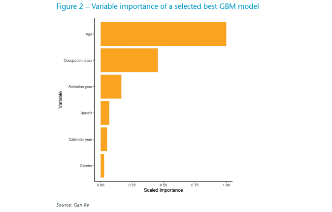
Variable importance can be also used to narrow down the number of variables that a refined pricing strategy could focus on.
Partial Dependence Plots (PDPs)
PDPs are a popular method that can be applied to visualise non-monotonic and non-linear patterns and to better understand the true contribution of variables (by averaging out the effect of other variables). They can also be used to enhance trust in the model’s outcome when the detected patterns and possible interactions between pairs of variables are in line with business reasonings and expectations.
PDPs can be interpreted in a similar way as interpreting coefficients in GLM models. For example, in Figure 3, we show how the average of modelled incidence rates changes in terms of “Calendar year” and “Selection year”, respectively. As it can be seen, unlike the observational data, incidence rates are rather constant in terms of “Calendar year” – when all confounding factors are considered.
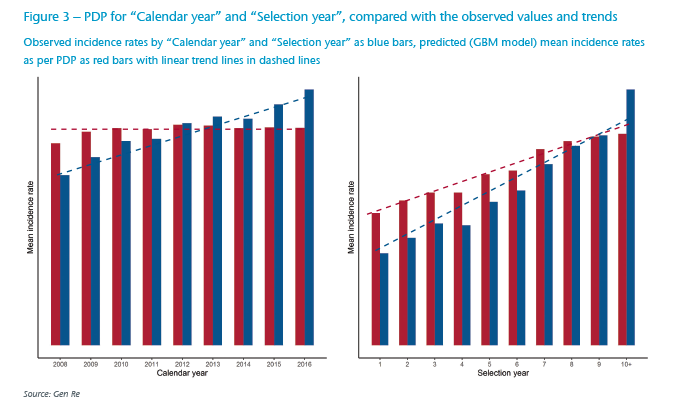
In contrast, there is a gradual increase with “Selection year” – but less prominent than what can be seen in pure observation, as the effect of other variables is not reflected. Thorough inspection of the data and discussions with experienced actuaries revealed that these are in fact the true underlying patterns, as an ageing portfolio impacts both “Calendar year” and “Selection year” effects.
Another advantageous application of PDPs is the ability to inspect the impact of two variables at the same time. In this way, characteristic behaviours, such as possible interactions and non-linear patterns, can easily be recognized. For example, in Figure 4, we show two-dimensional PDPs for “Occupation class” and “Age”.
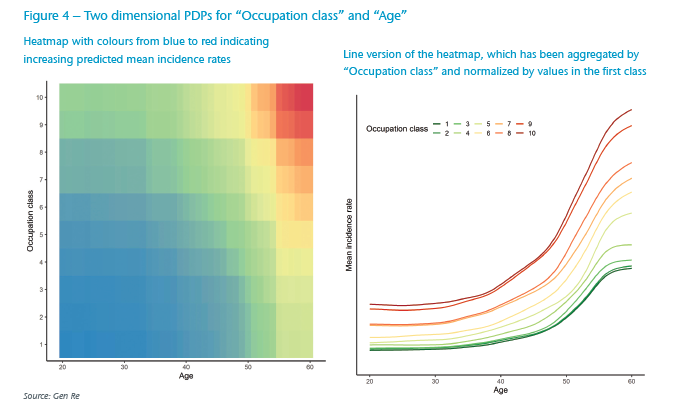
Figure 4 shows that average modelled incidence rates increase by “Age”, but customer segments in higher (riskier) “Occupation classes” start with higher rates and additionally the modelled incidence rates increase with a steeper slope by “Age”, i.e. a prominent interaction between “Age” and “Occupation class”.
Model deployment – calculating premiums with GBM rates
In this project, model deployment translated to calculating net risk and level premiums for various model points (MPs), potential applicants for a Disability Income policy (see Table 1). Given that our project is focused on incidence rates, we used a standard set of termination rates, which had been derived by traditional approaches and standard assumptions, which include, for example, the interest rate.
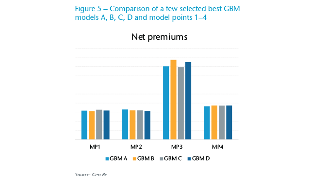
We applied the best GBM models directly to generate the output for the MPs, that is the incidence rates by “Age” and “Selection year” and transferred these into our normal pricing tools to generate technical level premiums as shown in Figure 5.
Integrating the results of pricing models derived by machine learning models into practical production systems would require additional finetuning, including documentation and further consistency checks to satisfy all regulations.
We also used this step as one last and most important step in our evaluation process: Calculating premiums with the top performing models should show consistent results and be reasonably comparable with traditional pricing approaches.
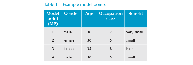
As we can see in Figure 5, the requirement of consistency is satisfied. MPs reflecting typical combinations in the data show very consistent net premiums across the top performing models. With rare combinations, such as in MP 3, the volatility in the raw data increases and this translates to slightly different model results, yet extrapolations or different smoothing approaches would generate a range of possible outcomes also with traditional approaches.
In contrast, a very typical combination such as MP 4, shows resulting net premium varying by less than 3%. A comparison with net premium calculated with a traditional approach showed a consistent overall picture with little differences, which could be explained when looking at the details of actuarial assumptions.
As the results are consistent within different top models, and are reasonably understandable compared with the traditional pricing analysis, this shows once more that the models and the entire approach satisfy our standards, and at the same time they improve insights and potential automation level of pricing tasks via machine learning.
Conclusion
In this article, we took one of the core actuarial tasks – technical pricing of Protection business – and designed a project applying state of the art methodological and technological approaches. We collected and iteratively revisited the data processing through the modelling steps in feedback loops. These feedback loops represent an important pre-requisite in transferring traditional data analysis to modern business-applicable AI solution.
We employed and extensively explored advanced analytics techniques. The advantage of these sophisticated algorithms is that besides linear and monotonic patterns, any possible non-linearity as well as complex interaction behaviour among variables can be recognized, with much less manual or ad-hoc assumptions. With rapid advances in the field of machine learning and widespread deployment of technology – for example, automated machine learning and cloud computing – these algorithms are quickly becoming a common approach.
Using our local supercomputer and H2O, a distributed and in-memory machine leaning platform, we constructed a multitude of models to identify top-performing models that describe the data best. In such mulitdimensional models, we generated more comprehensive insights, in contrast to pure data exploration, taking into account the contribution of all confounding variables at once.
Using interpretability methods, such as partial dependence plots, for the selected models we investigated and answered our business questions including “Calendar year” trend and the extent of “Selection year” effects. Detailed interactions between “Age” and “Occupation class” have also been recognized. Thanks to the transparency resulting from use of interpretability methods, we could also verify the consistency of predictions with actuarial expertise.
We used the top-performing models in production, applying the predicted incidence rates for selected potential insurance applicants for the course of their policy and used these in our actuarial premium calculation tools. We showed that the results are consistent among selected best models, especially interesting is that they vary very little for the most common combinations of variables and can easily serve as a refinement for traditional pricing approaches. We opened up further possibilities for pricing Protection business with adequate premiums that are commensurate with the risk of the individual.
Smart AI-based solutions that are deployed to automate tasks in an appropriately scalable infrastructure – such as a cloud environment or digital platforms – reduce timely and costly manual intervention and thus increase business efficiency and customer satisfaction by more personalised offerings.
At Gen Re we are at the forefront of AI applications in the Life and Health insurance business, and we are open to supporting and building innovative solutions with our clients.
Sources
- Ng, A., “How to choose your first AI project”, HBR, 2019: https://hbr.org/2019/02/how-to-choose-your-first-ai-project.
- H2O.ai, an open source machine learning platform https://www.h2o.ai/.
- Gen Re’s Dread Disease Survey and Insights From a Regional Analysis for China: https://www.genre.com/knowledge/publications/ri19-9-en.html.
- Hall, P. Gill, N., “An Introduction to Machine Learning Interpretability”, O’Reilly Media, 2019.


