-
Property & Casualty
Property & Casualty Overview

Property & Casualty
We offer a full range of reinsurance products and the expertise of our talented reinsurance team.
Expertise
Publication
Production of Lithium-Ion Batteries
Publication
Time to Limit the Risk of Cyber War in Property (Re)insurance
Publication
Generative Artificial Intelligence in Insurance – Three Lessons for Transformation from Past Arrivals of General-Purpose Technologies
Publication
Human Activity Generates Carbon and Warms the Atmosphere. Is Human Ingenuity Part of the Solution?
Publication
Inflation – What’s Next for the Insurance Industry and the Policyholders it Serves? -
Life & Health
Life & Health Overview

Life & Health
Gen Re’s valuable insights and risk transfer solutions help clients improve their business results. With tailor-made reinsurance programs, clients can achieve their life & health risk management objectives.
UnderwritingTraining & Education
Publication
The Key Elements of Critical Illness Definitions for Mental Health Disorders
Publication
What Are We to Make of Cannabis Use in The Insured Population? Business School
Publication
Knife or Needle: Will the New Weight Loss Medication Replace Bariatric Surgery?
Publication
Weight Loss Medication of the Future – Will We Soon Live in a Society Without Obesity? Moving The Dial On Mental Health
 -
Knowledge Center
Knowledge Center Overview

Knowledge Center
Our global experts share their insights on insurance industry topics.
Trending Topics -
About Us
About Us OverviewCorporate Information

Meet Gen Re
Gen Re delivers reinsurance solutions to the Life & Health and Property & Casualty insurance industries.
- Careers Careers
Unveiling Black Box Models – Interpretability and Trust

August 14, 2018
Dr. Behrang Jalali
English
Français
In most fields, domain-specific data analysis and generalized linear models (GLMs) have been routinely used to extract insights from the data. The underlying mathematics of such analyses are rather straightforward, and practitioners as well as non-technical project members are experienced in how to interpret the results, and thus are adept at applying them in the context of business.
In recent years more advanced models, including machine learning, have been increasingly applied and have been outperforming the traditional models. Machine learning models have been used in a wide range of applications, from image classification and text mining to customer segmentation and lapse analysis.
Machine learning models are usually known as black box models. This is due not only to the high degree of technical details needed to understand them but also to the results – for example, the recognised patterns between response and variables – that often cannot be formulated in terms of a concise relationship, whereas they can in linear models. But the capacity to recognise nonlinear and non-monotonic relationships between variables and response is precisely what sets these sophisticated models apart from traditional ones in performance terms.
Limited experience in applying such models and lack of access to easy-to-understand methods – for example, informative graphs, that communicate the results to non-technical members in a business context – prevents many practitioners and managers in implementing such models, especially in regulated industries such as life/health insurance.
This article introduces methods to help interpret the results (predictions) of machine learning models, and to better understand the models themselves. Additionally, these methods help evaluate the models in a business context, allowing project members to assess a model’s trustworthiness and requiring little technical expertise. The methods described can be implemented with all sorts of algorithms, and are therefore model-agnostic and can be used in both regression and classification applications.
The data and model
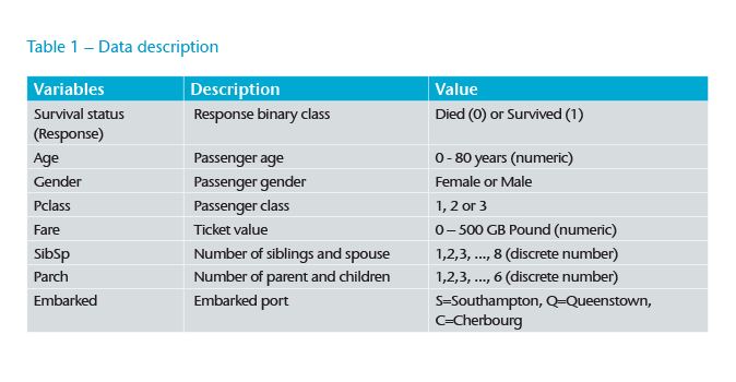
To illustrate the various methods, we use the generic Titanic data,1 representing the tragic accident of the Titanic passenger liner that more than 60% of passengers did not survive (see Table 1). We apply a Gradient Boosting Machine (GBM) as an example of a machine learning model. GBM is a tree-based model, and an ensemble of weak learners (models) that are sequentially built to construct the stronger final model. In this case, we use GBM as a binary classifier to model survival status of passengers.
Variable importance
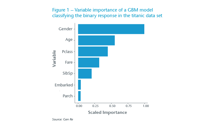
Variable importance is a list of all variables that have been included in a model, usually ranked in a descending order and it is statistically computed differently for specific machine learning models. Generally speaking, the more important variables cause a greater decrease in errors in describing the response variable (modelled survival status in this case). Figure 1 shows this list as the result of applying a GBM model using the Titanic data. In GLM models, this list can be similarly seen in terms of absolute values of coefficients, wherein the larger coefficients have higher impact (relative to other variables) in describing the response.
In the global scope, it is fundamentally useful to find out which variables are more important in a given project, and it is particularly useful in high dimensional data sets. It provides the first measure in assessing the trust of any model, which is established when the list of important variables is consistent with domain expectations and can also stay stable, with slight data variations. (Figure 1)
Partial dependence plot
The partial dependence plot (PDP) demonstrates the dependency of response on a variable or set of variables. It shows the marginal effect of the chosen variable on the response (for regression) or on the class probability (for classification). This effect is measured in changes in the mean response, e.g. for classification the change in class probability. I.e. the Y-axis no longer expresses the original response values. The idea can also be understood in analogy with interpreting coefficients in GLM models – in other words, how response is changing in terms of the chosen variable, assuming that the other variables are constant.
PDPs enhance trust when the results are consistent with the domain knowledge, and provide understanding of the model by visualizing nonlinearity and interactions.
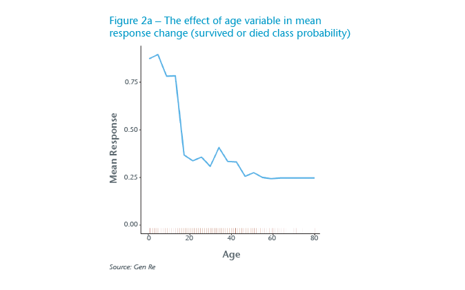
In Figure 2a, the left panel shows the dependency of response (Survived or Died class probability) with respect to the Age variable in modelling the Titanic data. We have added an extra feature to the shown PDPs that allows us to better decide how confident we can be across the Age range and cautiously take decisions if necessary. The added “rug” (small vertical ticks along the X-axes) shows that this data is too sparse after age of 60 years, particularly because very little data is available after the age 70.
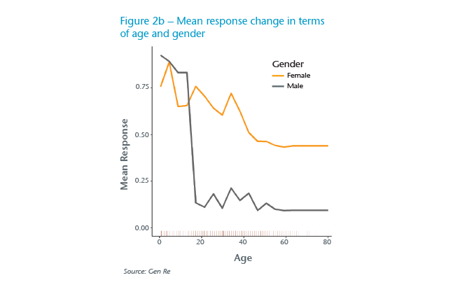
Using two variables, shown in the right panel in Figure 2b, PDP enables us to investigate the possible interaction between two variables in describing the behaviour of response. In this example, the existence of an interaction between the two variables is prominent. As can be seen, the mean survival probability is decreasing with Age (indicating that it is more likely older passengers do not survive), and also is higher for female passengers at any given Age. For Age below 15 years (children in this data), Age is a more important factor than Gender. The above interpretation is in line with reasonable assumptions that children and female passengers have been given priority to take to the lifeboats, consequently indicating that this model is trustworthy.
PDPs provide global information when considering the data as a whole, and are locally informative in terms of individual variables.
Surrogate models
Another method that helps interpret the results of machine learning models is to approximate the complex model predictions with a simpler, so-called surrogate model. The idea is to train a simple model, such as a linear regression or decision tree, with the original data but using predictions of the complex model as the response. Practically speaking, the simple model – which is less accurate than the actual complex model – is used to visualize and explain the patterns recognized.
Single decision tree
Figure 3 shows a trained decision tree, using the predicted probabilities of a GBM model as the response to visualize the recognized relations between the involved variables and response. Keep in mind the GBM model is itself an ensemble of 50 trees, and some of the trees in this case can be as deep as six levels.
Such easy-to-understand paths could be interpreted and used as business rules.
To read this tree, focus on the two far right-hand paths (marked in red). The first node at the top, the root, contains all the data used in this tree (100%) and shows the two probabilities, at this depth, for Died and Survived labels, 60% and 40% respectively. Moving to the second step, following the suggestion of the graph for female passengers (the “No” branch if Gender is not male), we move to the right orange node. Here we have 45% of all the data, i.e. those observations that have been predicted as Survived by 92% probability and just 8% probability for Died label. Up to this point, apart from the interpretation, the model is consistent with the historic information that female passengers are more likely to survive, and as a result this model seems trustworthy (for this branch). (see Figure 3)
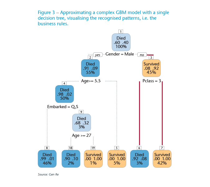
Continuing the above branch, for passengers in the third class (left split) the path ends at the last blue node (last node is called a leaf). There, 92% chance is for Died label. Similarly, for the right split ending at the orange leaf, it is suggested that observations representing female passengers in either of first or second class would certainly survive (100% Survived and 0% Died), and that contains 42% of the whole data.
Using a surrogate model also acts as a trust measure when the suggested rules are understandable according to the business background.
Surrogate models are beneficial in explaining graphically nonlinear and non-monotonic relations between variables and the response.
Approximating a complex model with a single decision tree can be considered applicable as a global interpretation as it describes average (or overall) contributions of variables to the predicted response. It can also be considered local when it is used to explain a decision path of a specific (group of) observation.
Note that there is no guarantee that this proxy would represent the complex model closely. In practice, it is necessary to experiment with the parameters of this method, and also to explore the distribution of predicted response (probabilities in the above example). In this example, we selected the observations that are modelled with high confidence, i.e. predicted probabilities closer to 0 and 1, aiming at revealing more prominent patterns.
Local interpretable model-agnostic explanations
Local interpretable model-agnostic explanations (LIME) provide an explanation for individual predictions by determining the most relevant (supportive or contradicting) variables of the given observations. This method was originally intended to be a model-agnostic interpretation approach for text and image classification. Its powerful capabilities were soon propagated to other applications, such as customer segmentation analysis.
LIME works essentially as the following: each observation (data row) is simulated by creating thousands of permutations. The trained complex model makes predictions based on these permutations. A simpler model, such as a linear regression, then models this generated data to find out the more important variables. The variables for each observation would be weighted based on a regression model, as can be seen in Figure 4 as an example for two randomly selected observations.
In Figure 4, the output of LIME is shown for two randomly selected observations (cases in LIME output) using the Titanic data shown. Both cases were selected from a sample of observations with correct predictions, meaning the observed response was correctly modelled. This exercise can also be done for wrong predictions (either false positive or false negative cases) to further explore those individual observations.
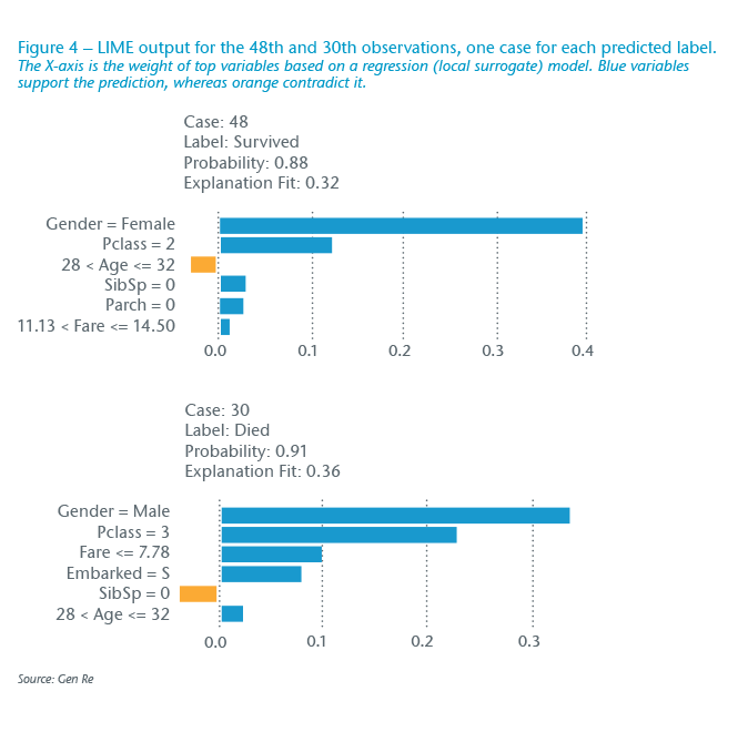
The upper panel shows the predicted label is Survived and has 88% probability, thus a confident prediction. We see that Gender (female in this observation) and passenger class (Pclass) have a large weight in determining this probability. These two variables, supporting the prediction outcome, are well aligned with the background of this accident. The fact that Age is weakly contradicting this prediction has little importance, considering its small weight in this observation. Looking into other variables in the list, having no family member could make taking to a lifeboat more likely, and apart from possibly small noise or fluctuations for negative small weight for Age, this recommendation is reasonable.
In the lower panel, we look at a predicted Died label. Here, a passenger who is male and in the third class (also with a very cheap Fare value), as well as being not too young a passenger, are reasonable arguments to correctly and confidently label this observation as Died.
By inspecting a meaningful fraction of individual cases, using LIME output, one should be able to:
- Assess the trustworthiness of the model
- Find out the top important variables that are common in supporting the correct predictions
- Better examine individual cases if needed for further business requirements, such as customer segmentation, claims and underwriting assessments
As can be expected in the aforementioned, this method is a local interpretation approach as there are local surrogate (linear) models for each observation.
Summary and conclusions
Machine learning models have a higher performance and wider range of applications compared with traditional analyses. Implementing these advanced models in the life cycle of analytics projects, in collaboration with domain experts, can certainly add value to the business.
In this article, we introduce model-agnostic techniques that offer more transparency in applying advanced models by enabling users to interpret results in a business context, and therefore enhance model understanding and trustworthiness.
These techniques can be applied to modelling of various applications in insurance, such as pricing, portfolio analysis, simplified underwriting, customer segmentation and claims analysis. Below are short descriptions of the proposed methods and how they help to interpret model results:
- Variable importance is an output list that describes the global contribution of included variables in modelling the response.
- Partial dependence plot (PDP) shows how the average modelled response changes in terms of the marginal effect of a specific variable. PDPs provide a powerful tool to visualize possible interactions, and can be useful to communicate the insights of any complex model to a non-technical audience.
- Surrogate models are simple models that approximate complex models to explain the recognized patterns, for example:
- A single decision tree can visually illustrate the path or business rules between the response and variables.
- LIME helps in exploring the rationale behind individual model predictions in that it provides variable importance at the local level.


